Sometimes I need to check bathymetric or topographic data. A good and fast way to do it is to use SURFER.
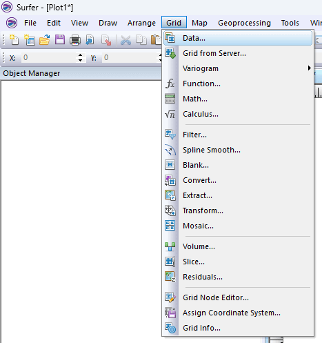
XYZ data need to be gridded first. Click Grid–>Data and open the file.
Select the file you want to be gridded or select the sheet that is already opened in Surfer
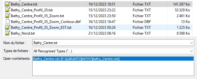
In the case you select a file, you have to import data as delimited text and then a windows pops up:
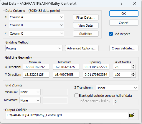
For an accurate work, this is the most important window. Depending on how your text file is organized select the right column to fit with XYZ data. Then the grinding method must be selected:
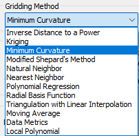
A lot of grinding methods exists. Kriging is the most popular. However, I often use minimum curvature that provide similar and faster results. Then the grinding Line Geometry defines the resolution of the map. Consider carefully this option.
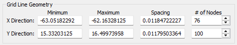
In the example above, data are in decimal degrees. By default, SURFER sts the spacing to 0.01 unit, meaning here that it’s 0.01 degree. So, the bin of the grid can be calculated, depending on the latitude. Please take a look at this article:
The data are located 15°N, meaning that the Longitude distance for 1° is 106 km and for 0.01° it’s 1.06 km. Depending on the initial resolution of data, the spacing must be set up. In my case it’s 0.001 to get a resolution of 100m.
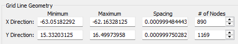
Reducing spacing increases the number of nodes (or cells). So it will drastically increase the calculation time. Once done, click of and wait.
In SURFER, open a new plot window and then click on Map–>New–>….
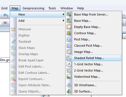
And select the kind of map you want to display.
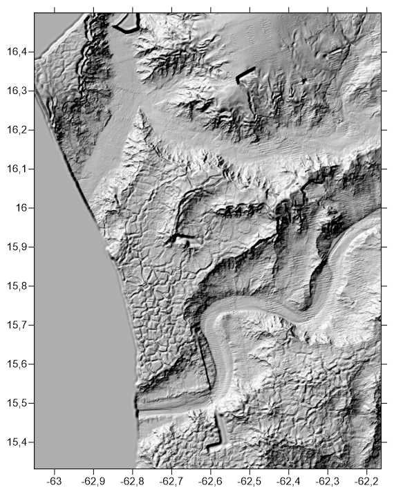
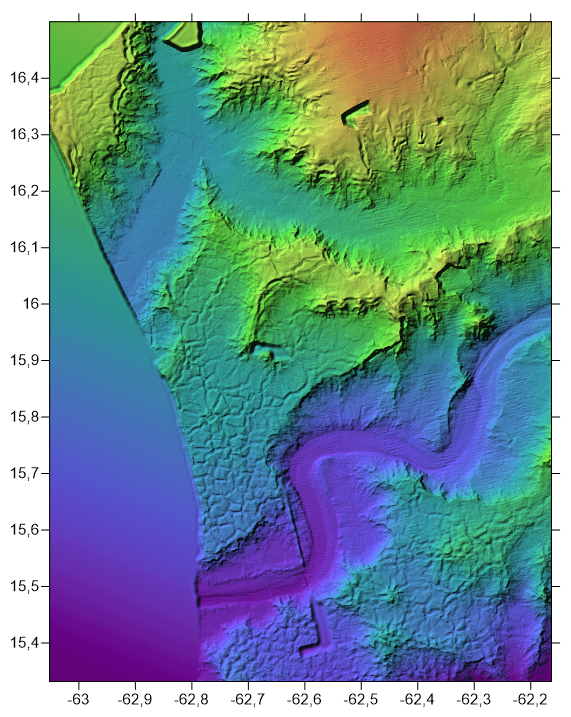
For instance, image map provide an aerial view from top with shaded relief:
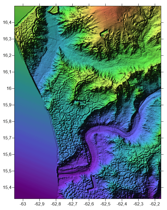
The shaded relief alone:
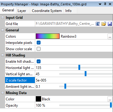
On the left pane, all options can be set up, particularly the colorbar and the vertical exaggeration (Z scale factor).
And the Map–>New–>3D Surface:
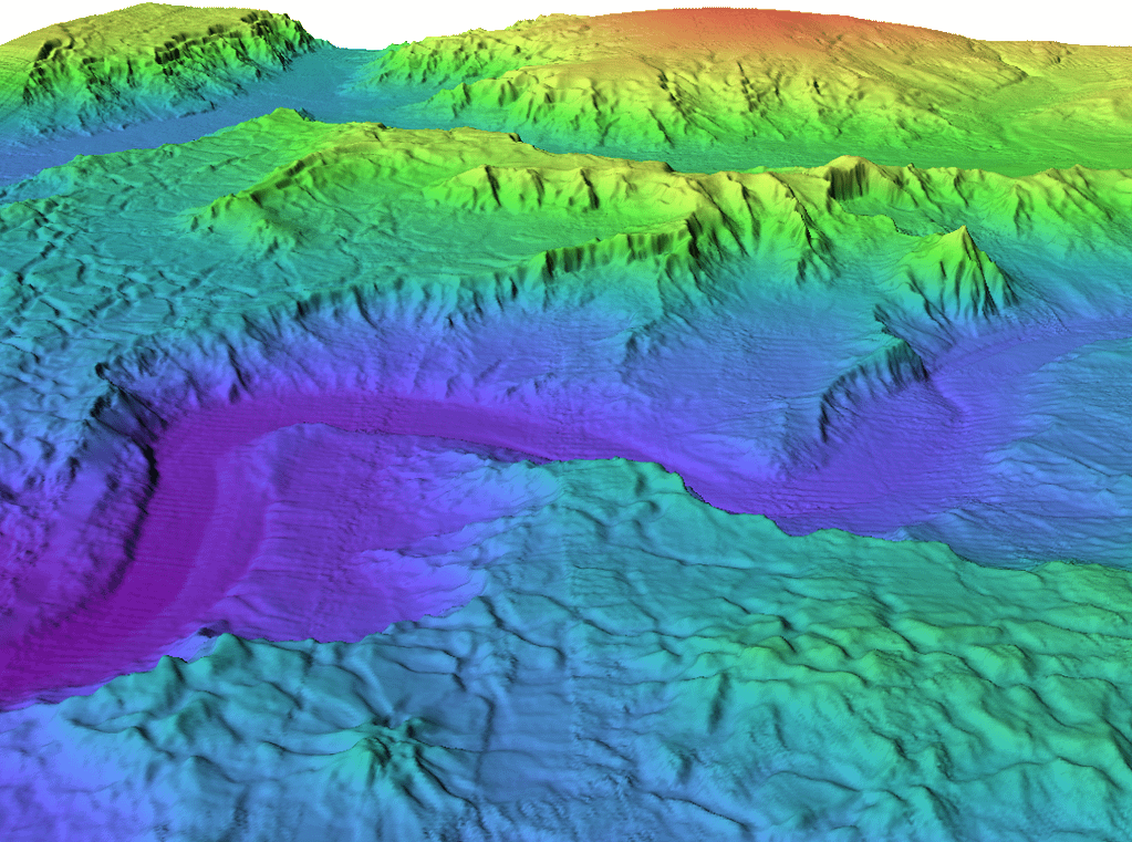
Let’s start interpretation 🙂